Audio : Listen to This Blog.
The Problem Statement
The Otto Product Classification Challenge was a competition hosted on Kaggle, a website dedicated to solving complex data science problems. The purpose of this challenge was to classify products into correct category, based on their recorded features.
Data
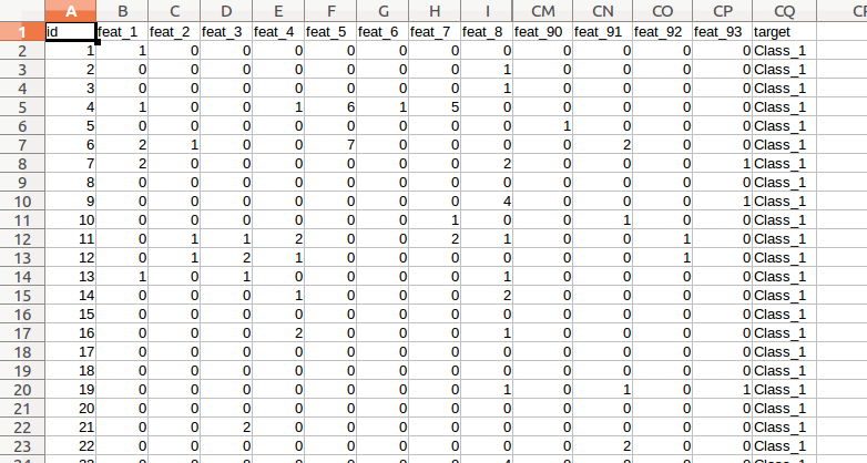
The organizers had provided a training data set containing 61878 entries, and a test data set that had 144368 entries. The data contained 93 features, based on which the products had to be classified. The target column in the training data set indicated the category of the product. The training and test data sets are available for download here. A sample of training data set can be seen in the figure 1.
Solution Approach
The features in the training data set had a large variance. Anscombe transform on the features reduced the variance. In the process, it also transformed the features from an approximately Poisson distribution into an approximately normal distribution. Rest of the data was pretty clean, and thus we could use it directly as input to the classification algorithm. For classification, we tried two approaches { one was using the xgboost algorithm, and other using the deeplearning algorithm through h2o. xgboost is an implementation of extreme gradient boosting algorithm, which can be used effectively for classification.

Figure 1: Sample Data
As discussed in the TFI blog, The gradient boosting algorithm is an ensemble method based on decision trees. For classification, at every branch in the tree, it tries to eliminate a category, to finally have only one category per leaf node. For this, it needs to build trees for each category separately. But since we had only 9 categories, we decided to use it. The deep learning algorithm provided by h2o is based on a multi-layer neural network. It is trained using a variation of gradient descent method. We used multi-class logarithmic loss as the error metric to find a good model, as this was also the model used for ranking by Kaggle.
Building the Classifier
Initially, we created a classifier using xgboost. The xgboost configuration for our best submission is as below:
param list(`objective' = `multi:softprob',
`eval metric' = `mlogloss', `num class' = 9,
`nthread' = 8, `eta'= 0.1,
`max depth' = 27, `gamma' = 2,
`min child weight' = 3, `subsample' = 0.75,
`colsample bytree' = 0.85)
nround = 5000
classi�er = xgboost(param=param, data = x, label = y, nrounds=nround)
Here, we have specified our objective function to be multi:softprob’. This function returns the probabilities for a product being classified into a specific category. Evaluation metric, as specified earlier, is the multiclass logarithmic loss function. The eta’ parameter shrinks the priors for features, thus making the algorithm less prone to overfitting. The parameter usually takes values between 0:1 to 0:001. The max depth’ parameter will limit the height of the decision trees. Shallow trees are constructed faster. Not specifying this parameter lets the trees grow as deep as required. The min child weight’ controls the splitting of the tree. The value of the parameter puts a lower bound on the weight of each child node, before it can be split further. The subsample’ parameter makes the algorithm choose a subset of the training set. In our case, it randomly chooses 75% of the training data to build the classifier. The colsample bytree’ parameter makes the algorithm choose a subset of features while building the tree, in our case to 85%. Both subsample’ as well as colsample bytree’ help in preventing over t. The classier was built by performing 5000 iterations over the training data set. These parameters were tuned by experimentation, by trying to minimize the log-loss error. The log-loss error on public leader board for this configuration was 0.448.
We also created another classifier using the deep-learning algorithm provided by h2o. The configuration for this algorithm was as follows:
classi�cation=T,
activation=`Recti�erWithDropout',
hidden=c(1024,512,256),
hidden dropout ratio=c(0.5,0.5,0.5),
input dropout ratio=0.05,
epochs=50,
l1=1e-5,
l2=1e-5,
rho=0.99,
epsilon=1e-8,
train samples per iteration=4000,
max w2=10,
seed=1
This configuration creates a neural network with 3 hidden layers, each with 1024, 512 and 256 neurons respectively. This is specified using the `hidden’ parameter. The activation function in this case is Rectifier with Dropout. The rectifier function filters negative inputs for each neuron. Dropout lets us randomly drop inputs to the hidden neuron layers. Dropout builds better generalizations. The hidden_dropout _ratio specifies the percentage of inputs to hidden layers to be dropped. The input dropout ratio specifies the percentage of inputs to the input layer to be dropped. Epochs define the number of training iterations to be carried out. Setting train samples per iteration makes the algorithm choose subset of training data. Setting l1 and l2 scales the weights assigned to each feature. l1 reduces model complexity, and l2 introduces bias in estimation. Rho and Epsilon together slow convergence. The max w2 function sets an upper limit on the sum of squared incoming weights into a neuron. This needs to be set for rectifier activation function. Seed is the random seed that controls sampling. Using these parameters, we performed 10 iterations of deep learning, and submitted the mean of the 10 results as the output. The log-loss error on public leaderboard for this con figuration was 0.448.
We then merged both the results by taking a mean, and that resulted in the top 10% submission, with a score of 0.428.
Results
Since the public leaderboard evaluation was based on 70% of the test data, the public leaderboard rank was fairly stable. We submitted the best two results, and our rank remained in the top 10% at the end of final evaluation. Overall, it was a good learning experience.
What We Learnt
Relying on results of one model may not give the best possible result. Combining results of various approaches may reduce the error by significant margin. As can been seen here, the winning solution in this competition had a much more complex ensemble. Complex ensembles may be the way ahead for getting better at complex problems like classification.


